Table of Contents
Problem Description
Mathematical Formulation
Solver Description
Results
Source Code
Problem Description
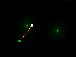
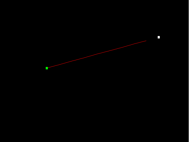
The goal of this project is to find out if optimization can solve projectile path planning problems, especially when the projectile is influenced by forces that vary across space. Specifically, given a start and end point and a finite time for the flight of the projectile, we want to compute its trajectory. In my implementation, the green dot and red dot represent the desired and end positions. The space that the projectile flies in, can have different fields - gravity can be toggled on/off along either axis, and blackholes (potential fields) can be created at arbitrary locations. The force acting on the particle due to a potential field is obtained by taking the gradient of the field at that position.
The optimization problem is formulated similar to other spacetime problems in animation. The domain of the problem is the set of positions of the projectile at each time step. The positions are constrained by the physics of the problem (i.e the sum of forces on the projectile must be zero) as well as the the specified start and end positions. These constraints are folded into an objective function that can then be minimized using a Quasi-Newton optimization.
It is important to note that introducing arbitrary potential fields can make this a non-convex problem and the optimization may find a local minima that violates some of these constraints. However, simple constant gravitational fields retain convexity and result in global minima.
Mathematical Formulation
Since the final project requires me to use a Quasi-Newton optimization, all constraints must be eliminated. These constraints all happen to be equality constraints (force balance and position specifications) and can be folded into the objective (y) by representing them as a sum of squares.
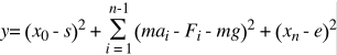
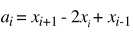
where each Xi denotes the position at timestep i, and Fi represents the external force at Xi and s,e represent start and end positions. Acceleration can be represented in terms of position using finite differencing. The domain consists of all Xi.

We minimize objective function y using a Rank Two Quasi Newton method described in the next section. The result is a vector of positions of the projectile at each time step. The gradient is computed by differentiating the objective function with respect to each Xi and is an inexpensive operation.
Solver Description
Quasi Newton (QN) methods are typically used to handle non-linear unconstrained optimization problems. They are similar to Conjugate Gradient (CG) techniques, but do not require a Hessian to be provided. Instead, they build up curvature information progressively by using new gradient data. Hence at each step, an approximation of the Hessian is obtained. One should note that while some variants of CG (Fletcher-Reeves) do not force the Hessian requirement either, they do not create this Hessian approximation and as a result, QN methods are rather useful in this regard.
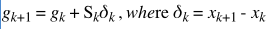
Mathematically, the QN method is derived as follows. In gradient based searches, the kth iteration is given by:

where Sk is typically the Hessian for CG methods. Suppose Sk was instead a nxn positive definite matrix, we can find a value for alpha that minimizes the objective function. The closer S is to H, the more accurate is the solution. In order to approximate H, S is updated each iteration using gradient information. The basis for this is the Taylor expansion of the gradient:
Depending on the type of update used, Ck is either a rank 1 or 2 matrix. We solve for Ck by solving this equation (obtained from the Taylor expansion):
The details of the solution of this system of equations has been omitted here but the result gives the new value of the S matrix, which is then used in the next step for the line search. It is desirable to have the search directions to be conjugate in each step as well as a positive definite Sk.
Results
Since this was largely an experiment to find out if unconstrained optimization can solve this problem, I was quite thrilled to see some of these results. This uses the BFGS Rank 2 Quasi Newton optimizer written by Kane Bonnette. The red line shows the positions obtained from the optimization while the yellow line is obtained by simulating the projectile by computing acceleration at each time step, while using only the initial velocity obtained from the optimization. There is one caveat to this approach for comparing results - namely the assumption that the initial velocity is correct. Still, it helps to verify that the path predicted by the optimization is exactly the one it will take if launched with that velocity (in the case of uniform gravitational fields).
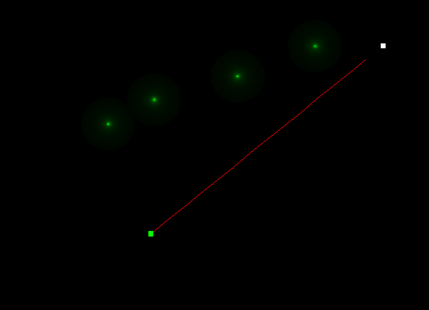
First, I verified that the formulation of the gradient and objective functions were correct by releasing the projectile in a space without any external forces. As expected, the projectile travels in a straight line towards the target.
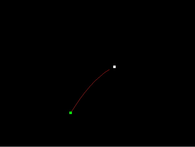
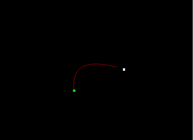
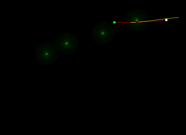
Next, I tested it with gravitational fields along X, then along Y and then along both. Again, this produces perfect results (paraboloids):
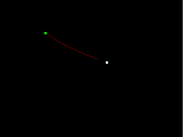
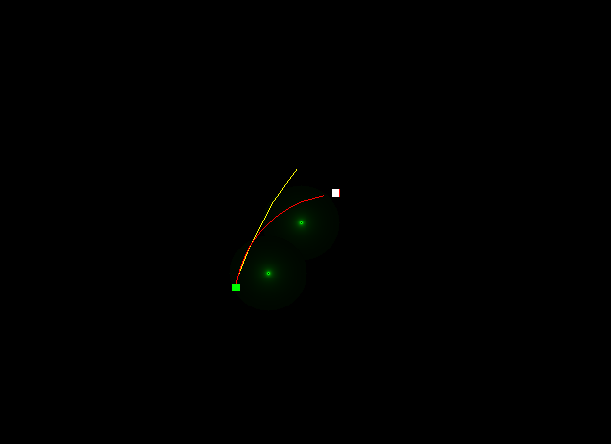
To make things more interesting, I added black holes. These draw the projectile towards the center when it gets with their range. This makes the problem non-convex and also discontinuous at points. I was able to obtain the following results. First, the good ones:
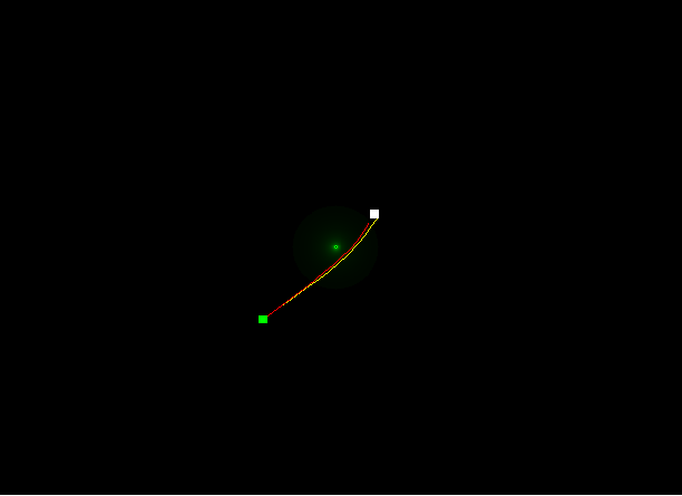
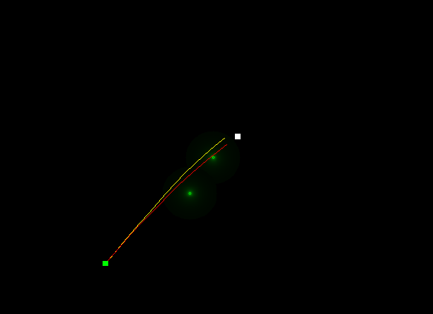
And some really poor ones:
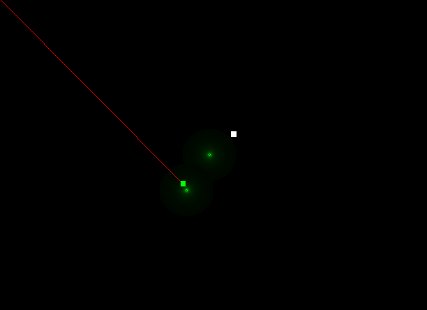
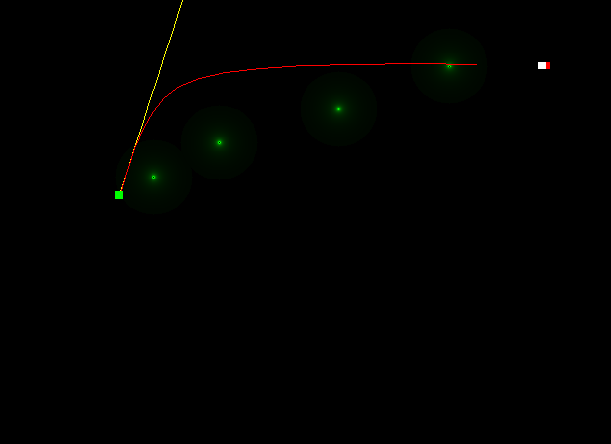
My best guess as to why some trajectories deviate so much from the simulated ones is that the optimizer has found some local minima that satisfy only some of the constraints fully. Having the centre of the black hole very close to the start or end points results in a very high initial velocity and causes the optimizer to fail.
In terms of performance, for simple gravitational fields, the optimization achieves an error of less than 1e-5 in about 50 iterations for 10 time steps. It is about linear in performance with the timesteps in this regard, and achieves the same error in about 120 iterations for 20 timesteps and 160 iterations for 30 timesteps.
Adding blackholes generally causes greater number of iterations unless the trajectory is not affected by them. However, it appears that poor results usually are accompanied with lower number of iterations indicating that the optimizer found some local minima.
In conclusion, I think this optimization approach obtains results for most reasonable configurations of black holes. However, I am unable to explain the strange behaviour in some cases and these could be the result of a highly non-convex objective function or due to discontinuities because of the potential field. I had attempted to allow user sketched fields based on the distance transform but that caused a greater number of discontinuities. It would be interesting to try this problem with a smoothed field as well as other optimization techniques.
Source Code
The source code for this project can be downloaded here . It is intended to be built on Linux although I'm fairly sure that you can build it using Cygwin. You will need the GNU Scientific Library to be installed and it can be downloaded from here . You will also need GLUT to be installed (default on many Linux distributions). To compile, type make.
To use this program: Press 'x' to toggle gravitational field along X on/off. Press 'y' to do the same to the field along Y. Press 's' and click to define start point. Press 'e' and click to define the end point. Press 'b' and click to place a black hole. Press 'c' to clear all blackholes. Hit the Spacebar to run the simulation. You might need to install graphics driver for a smooth simulation - virtual machines can run the application but mouse movement tends to be rather sticky.